Econometrics by Example 2nd Edition Gujarati Solutions Manual
You may also like
This is completed downloadable of Econometrics by Example 2nd Edition Gujarati Solutions Manual
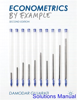
Product Details:
- ISBN-10 : 1137375019
- ISBN-13 : 978-1137375018
- Author:
The second edition of this bestselling textbook retains its unique learning-by-doing approach to econometrics. Rather than relying on complex theoretical discussions and complicated mathematics, this book explains econometrics from a practical point of view by walking the student through real-life examples, step by step. Damodar Gujarati’s clear, concise, writing style guides students from model formulation, to estimation and hypothesis-testing, through to post-estimation diagnostics. The basic statistics needed to follow the book are covered in an appendix, making the book a flexible and self-contained learning resource.
Table of Content:
- Part I: Basics of linear regression
- 1. The linear regression model: an overview
- 1.1 The linear regression model
- 1.2 The nature and sources of data
- 1.3 Estimation of the linear regression model
- 1.4 The classical linear regression model (CLRM)
- 1.5 Variances and standard errors of OLS estimators
- 1.6 Testing hypotheses about the true or population regression coefficients
- 1.7 R2: a measure of goodness of fit of the estimated regression
- 1.8 An illustrative example: the determinants of hourly wages
- 1.9 Forecasting
- 1.10 The road ahead
- Exercises
- Appendix: The method of maximum likelihood (ML)
- 2. Functional forms of regression models
- 2.1 Log-linear, double log or constant elasticity models
- 2.2 Testing validity of linear restrictions
- 2.3 Log-lin or growth models
- 2.4 Lin-log models
- 2.5 Reciprocal models
- 2.6 Polynomial regression models
- 2.7 Choice of the functional form
- 2.8 Comparing linear and log-linear models
- 2.9 Regression on standardized variables
- 2.10 Regression through the origin: the zero-intercept model
- 2.11 Measures of goodness of fit
- 2.12 Summary and conclusions
- Exercises
- 3. Qualitative explanatory variables regression models
- 3.1 Wage function revisited
- 3.2 Refinement of the wage function
- 3.3 Another refinement of the wage function
- 3.4 Functional form of the wage regression
- 3.5 Use of dummy variables in structural change
- 3.6 Use of dummy variables in seasonal data
- 3.7 Expanded sales function
- 3.8 Piecewise linear regression
- 3.9 Summary and conclusions
- Exercises
- Part II : Regression diagnostics
- 4. Regression diagnostic I: multicollinearity
- 4.1 Consequences of imperfect collinearity
- 4.2 An example: married women’s hours of work in the labor market
- 4.3 Detection of multicollinearity
- 4.4 Remedial measures
- 4.5 The method of principal components (PC)
- 4.6 Summary and conclusions
- Exercises
- 5. Regression diagnostic II: heteroscedasticity
- 5.1 Consequences of heteroscedasticity
- 5.2 Abortion rates in the USA
- 5.3 Detection of heteroscedasticity
- 5.4 Remedial measures
- 5.5 Summary and conclusions
- Exercises
- 6. Regression diagnostic III: autocorrelation
- 6.1 US consumption function, 1947–2000
- 6.2 Tests of autocorrelation
- 6.3 Remedial measures
- 6.4 Model evaluation
- 6.5 Summary and conclusions
- Exercises
- 7. Regression diagnostic IV: model specification errors
- 7.1 Omission of relevant variables
- 7.2 Tests of omitted variables
- 7.3 Inclusion of irrelevant or unnecessary variables
- 7.4 Misspecification of the functional form of a regression model
- 7.5 Errors of measurement
- 7.6 Outliers, leverage and influence data
- 7.7 Probability distribution of the error term
- 7.8 Random or stochastic regressors
- 7.9 The simultaneity problem
- 7.10 Dynamic regression models
- 7.11 Summary and conclusions
- Exercises
- Appendix: Inconsistency of the OLS estimators of the consumption function
- Part III : Topics in cross-section data
- 8. The logit and probit models
- 8.1 An illustrative example: to smoke or not to smoke
- 8.2 The linear probability model (LPM)
- 8.3 The logit model
- 8.4 The language of the odds ratio (OR)
- 8.5 The probit model
- 8.6 Summary and conclusions
- Exercises
- 9. Multinomial regression models
- 9.1 The nature of multinomial regression models
- 9.2 Multinomial logit model (MLM): school choice
- 9.3 Conditional logit model (CLM)
- 9.4 Mixed logit (MXL)
- 9.5 Summary and conclusions
- Exercises
- 10. Ordinal regression models
- 10.1 Ordered multinomial models (OMM)
- 10.2 Estimation of ordered logit model (OLM)
- 10.3 An illustrative example: attitudes toward working mothers
- 10.4 Limitation of the proportional odds model
- 10.5 Summary and conclusions
- Exercises
- Appendix: Derivation of Eq. (10.4)
- 11. Limited dependent variable regression models
- 11.1 Censored regression models
- 11.2 Maximum likelihood (ML) estimation of the censored regression model: the Tobit model
- 11.3 Truncated sample regression models
- 11.4 A concluding example
- 11.5 Summary and conclusions
- Exercises
- Appendix: Heckman’s (Heckit) selection-bias model
- 12. Modeling count data: the Poisson and negative binomial regression models
- 12.1 An illustrative example
- 12.2 The Poisson regression model (PRM)
- 12.3 Limitation of the Poisson regression model
- 12.4 The Negative Binomial Regression Model (NBRM)
- 12.5 Summary and conclusions
- Exercises
- Part IV : Time series econometrics
- 13. Stationary and nonstationary time series
- 13.1 Are exchange rates stationary?
- 13.2 The importance of stationary time series
- 13.3 Tests of stationarity
- 13.4 The unit root test of stationarity
- 13.5 Trend stationary vs. difference stationary time series
- 13.6 The random walk model (RWM)
- 13.7 Summary and conclusions
- Exercises
- 14. Cointegration and error correction models
- 14.1 The phenomenon of spurious regression
- 14.2 Simulation of spurious regression
- 14.3 Is the regression of consumption expenditure on disposable income spurious?
- 14.4 When a spurious regression may not be spurious
- 14.5 Tests of cointegration
- 14.6 Cointegration and error correction mechanism (ECM)
- 14.7 Are 3-month and 6-month Treasury Bill rates cointegrated?
- 14.8 Summary and conclusions
- Exercises
- 15. Asset price volatility: the ARCH and GARCH models
- 15.1 The ARCH model
- 15.2 The GARCH model
- 15.3 Further extensions of the ARCH model
- 15.4 Summary and conclusions
- Exercises
- 16. Economic forecasting
- 16.1 Forecasting with regression models
- 16.2 The Box–Jenkins methodology: ARIMA modeling
- 16.3 An ARMA model of IBM daily closing prices, 3 January 2000 to 31 October 2002
- 16.4 Vector autoregression (VAR)
- 16.5 Testing causality using VAR: the Granger causality test
- 16.6 Summary and conclusions
- Exercises
- Appendix: Measures of forecast accuracy
- Part V: Selected topics in econometrics
- 17. Panel data regression models
- 17.1 The importance of panel data
- 17.2 An illustrative example: charitable giving
- 17.3 Pooled OLS regression of charity function
- 17.4 The fixed effects least squares dummy variable (LSDV) model
- 17.5 Limitations of the fixed effects LSDV model
- 17.6 The fixed effect within group (WG) estimator
- 17.7 The random effects model (REM) or error components model (ECM)
- 17.8 Fixed effects model vs. random effects model
- 17.9 Properties of various estimators
- 17.10 Panel data regressions: some concluding comments
- 17.11 Summary and conclusions
- Exercises
- 18. Survival analysis
- 18.1 An illustrative example: modeling recidivism duration
- 18.2 Terminology of survival analysis
- 18.3 Modeling recidivism duration
- 18.4 Exponential probability distribution
- 18.5 Weibull probability distribution
- 18.6 The proportional hazard model
- 18.7 Summary and conclusions
- Exercises
- 19. Stochastic regressors and the method of instrumental variables
- 19.1 The problem of endogeneity
- 19.2 The problem with stochastic regressors
- 19.3 Reasons for correlation between regressors and the error term
- 19.4 The method of instrumental variables
- 19.5 Monte Carlo simulation of IV
- 19.6 Some illustrative examples
- 19.7 A numerical example: earnings and educational attainment of youth in the USA
- 19.8 Hypothesis testing under IV estimation
- 19.9 Test of endogeneity of a regressor
- 19.10 How to find whether an instrument is weak or strong
- 19.11 The case of multiple instruments
- 19.12 Regression involving more than one endogenous regressor
- 19.13 Summary and conclusions
- Exercises
- 20. Beyond OLS: quantile regression
- 20.1 Quantiles
- 20.2 The quantile regression model (QRM)
- 20.3 The quantile wage regression model
- 20.4 Median wage regression
- 20.5 Wage regressions for 25%, 50% and 75% quantiles
- 20.6 Test of coefficient equality of different quantiles
- 20.7 Summary of OLS and 25th, 50th (median) and 75th quantile regressions
- 20.8 Quantile regressions in Eviews 8
- 20.9 Summary and conclusions
- Exercises
- Appendix: The mechanics of quantile regression
- 21. Multivariate regression models
- 21.1 Some examples of MRMs
- 21.2 Advantages of joint estimation
- 21.3 An illustrative example of MRM estimation with the same explanatory variables
- 21.4 Estimation of MRM
- 21.5 Other advantages of MRM
- 21.6 Some technical aspects of MRM
- 21.7 Seemingly Unrelated Regression Equations (SURE)
- 21.8 Summary and conclusions
- Exercises
- Appendix
- Appendices
- 1. Data sets used in the text
- 2. Statistical appendix
- A.1 Summation notation
- A.2 Experiments
- A.3 Empirical definition of probability
- A.4 Probabilities: properties, rules, and definitions
- A.5 Probability distributions of random variables
- A.6 Expected value and variance
- A.7 Covariance and correlation coefficient
- A.8 Normal distribution
- A.9 Student’s t distribution
- A.10 Chi-square (??2) distribution
- A.11 F distribution
- A.12 Statistical inference
- Exercises
- Exponential and logarithmic functions
- Index
People Also Search:
econometrics by example gujarati
econometrics by example 2nd edition gujarati
econometrics by example 2nd edition
econometrics by example
econometrics by example 2nd edition download scribd
econometrics by example 2nd edition solution manual download pdf

